PCA is a dimensionality reduction framework in machine learning. According to Wikipedia, PCA (or Principal Component Analysis) is a “statistical procedure that uses orthogonal transformation to convert a set of observations of possibly correlated variables…into a set of values of linearly uncorrelated variables called principal components.”

The Benefits of PCA (Principal Component Analysis)

PCA is an unsupervised learning technique that offers a number of benefits. For example, by reducing the dimensionality of the data, PCA enables us to better generalize machine learning models. This helps us deal with the “curse of dimensionality” [1].

Algorithm performance typically depends on the dimension of the data. Models running on high-dimensional data might perform very slowly or even fail, requiring significant server resources. PCA can help us improve performance at a meager cost of model accuracy.

Other benefits of PCA include reduction of noise in the data, feature selection (to a certain extent), and the ability to produce independent, uncorrelated features of the data. PCA also allows us to visualize data and allow for the inspection of clustering/classification algorithms. 

A Closer Look at PCA (Principal Component Analysis)

Let’s examine the model to help us further describe PCA. It assumes that we have a high-dimensional representation of data that is, in fact, embedded in a low-dimensional space. We assume that L≈XV where L is some low-rank matrix, X is the original data and V is a projection operator.

Our original data has n features, and we wish to reduce them to k features, where k << n. With this, we need to project the data onto another vector space [2].

PCA has many interesting representations, but we’ll look at a formulation that we’ve found to be the most natural:

• To find the Principal Components (PCs), we wish to minimize the squared reconstruction error between our original data points and their projection onto some k-dimensional vector space.
• Mathematically, we need to find a projection matrix V that solves the following optimization problem:argminVTV=Ik‖X−XVVT‖F2‍
• X is our original data. XV is the projection to the k-dimensional space, and XVV is the reconstruction back to the original space.
• Projection from a 2-dimensional space to a 1-dimensional space can be illustrated by the following image:

In the image above:

• The blue dots are our original data vectors.
• The red dots are their projections.
• The blue lines are the reconstruction errors.
• The dashed black line is the optimal projection V that we found when solving our optimization problem.

We have now successfully projected the data from a 2-dimensional space (x,y axis) to a 1-dimensional space (line).

How PCA Maximizes the Variance of Data

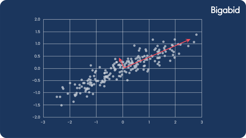
You might have heard something about PCA maximizing the variance of data. This is also true. Equivalence can be shown between the PCA problem we presented and the following formulation: 

argmaxWTW=IkWT(XTX)W

This captures as much variance in the data as possible since XX is proportional to the data covariance matrix.

This is illustrated by the following image, where we are maximizing the variance (distribution) along the projection axis:

How to Perform PCA (Principal Component Analysis)

In practice, PCA is usually solved using Eigenvalue Decomposition [3] as this is computationally efficient. While many Python packages include built-in functions to perform PCA, let’s take what we’ve just learned in order to implement PCA:

#Setup
import numpy as np
from numpy import linalg as la
from sklearn.preprocessing import StandardScaler
#Inputs:
# A – data matrix of order m X n
# n_components – how many principal components to return
#Returns: first n principal components + their explained variance + a transformed data matrix
def custom_pca(A, n_components=None):

    if n_components is None:
        n_components = A.shape[1]

    n = A.shape[1]
    B = StandardScaler().fit_transform(A) #scale and centre the data
    C = 1/(n-1) * (B.T @ B)               #create cov matrix
    eigvalues, eigvectors = la.eig(C)     #get the principal components
    idx = eigvalues.argsort()[::-1]       #Sort eigenvectors
    eigvalues = eigvalues.real[idx]       #Take only real vectors
    eigvectors = eigvectors.real[:,idx]

    explained_var = []                    #get the explained variance
    for i in range(n_components):
        temp_var = eigvalues[i] / np.sum(eigvalues)
        explained_var = np.append(explained_var, temp_var)
A_Projected = B @ eigvectors[:,:n_components] #project the data
return eigvectors.T[0:n_components], explained_var[0:n_components + 1], A_Projected

You can also implement PCA using sklearn:

from sklearn.decomposition import PCA
pca = PCA() #select the model
pca.fit(X)  #fit the model
PCs = pca.components_ #get the principal components vectors
exp_var = pca.explained_variance_ #get the explained variance
X_projected = pca.transform(X)  #project the data

Note that sklearn does not scale the data, it only centers it. Therefore, you might receive different results between the methods. However, since the method is influenced by the variables’ scale, scaling is important [4].

Also, don’t forget to look at the explained variance vector, as it will help you choose the right number of components. While there is no accurate rule for it, when you see the slope of the variance plotting flattens significantly, this is the time to stop. 

Let’s see an example of such an explained variance plotting. In this case, we could stop at 4 / 5 components:

PCA Use Cases

Example 1: Improve Algorithm Runtime

• KNN is a popular machine learning classifier, however its performance can be slow.
• In the next example, we produced a classification dataset of 1M records with 200 features. Only 5 of them informative.
• KNN ran for ~22 seconds on the full dataset. Running KNN after projecting the data to a 5-dimensional space took only ~1 second! (running on a MacBookPro, 2.3 GHz Intel Core i5, 8GB RAM)
• Here is the code we ran:

#setup
import time
from sklearn import datasets, neighbors
from sklearn.model_selection import train_test_split
#create dataset
data, labels = datasets.make_classification(n_samples=100000, n_features=200, n_informative=5 , n_redundant=195, n_classes=2, random_state=42)
#project the data
data_projected = custom_pca(data, n_components=5)[2]
#train-test split
X_train_full, X_test_full, y_train, y_test = train_test_split(data, labels, test_size=0.3, random_state=42)
X_train_proj, X_test_proj, y_train, y_test = train_test_split(data_projected, labels, test_size=0.3, random_state=42)
#run classifier on full data
clf = neighbors.KNeighborsClassifier()
clf.fit(X_train_full, y_train)
tic = time.perf_counter()
predictions = clf.predict(X_test_full)
runtime_full = time.perf_counter() – tic
print(‘full model ran in’, round(runtime_full, 2), ‘seconds’)
#run classifier on PCA data
clf.fit(X_train_proj, y_train)
tic = time.perf_counter()
predictions = clf.predict(X_test_proj)
runtime_proj = time.perf_counter() – tic
print(‘PCA model ran in’, round(runtime_proj, 2), ‘seconds’)

• The model accuracy remained the same (check it!)
• In this example, we knew a-priori that the data is “really” 5-dimensional. But plotting the explained variance vector could anyway help us figure out how many PCs we needed.

Example 2: Improve Classification Accuracy

The following article demonstrates an improvement to the accuracy of the tree classifier C4.5 using PCA. Running an experiment on a medical dataset from UCI Machine Learning repository, the authors we able to improve model accuracy from 86% to 91% while precision dramatically improved from 33% to 100%. 

In another article, the authors analysed the performance of six different machine learning classifiers. They were able to get improvement in accuracy while reducing the number of features from over 1000 to just a few principal components.

Example 3: Visualization

• The famous iris dataset is 4-dimensional. Unfortunately, we cannot visualize data with more than 3 features.
• Using PCA, we projected the data to a 2-dimensional space:
• This is very helpful for presenting data to various people in your organization. Moreover, it makes it possible to visualize and inspect clustering and classification algorithms and their performance. 

Example 4: Reduce Noise in Data

• To demonstrate reduction in noise, let’s look at the following example:

• The data is mostly spread along the x-axis, while on the y-axis the distribution is dominated more by noise. 
• Projecting the data to a 1-dimensional space eliminates that noise.
• Using PCA to clean noise from data that represents a signal (image, audio) can help achieve a “cleaner” signal.

Example 5: Feature Selection

For feature selection, consider that in the previous example, the first principal component vector is (0.905, 0.423). This means that the projection is a linear combination of the two features with ratio of approximately 2:1. We could use this knowledge in order to perform feature selection. The features we see that get most weight of the projection in the primary principal components are the important features. We could use that fact in order to run models on our original data (without PCA transformation), and by doing so, maintain interpretability of the model.

Drawbacks of PCA (Principal Component Analysis)

As with any framework, PCA has its own drawbacks. First, PCA assumes that the relationship between variables are linear. If the data is embedded on a nonlinear manifold, PCA will produce wrong results [5].

PCA is also sensitive to outliers. Such data inputs could produce results that are very much off the correct projection of the data [6].

PCA presents limitations when it comes to interpretability. Since we’re transforming the data, features lose their original meaning. This could be problematic in cases where interpretability of the data is important. However, in the feature selection example we mentioned earlier, there are cases where we can still partially interpret the model. 

Finally, PCA is only suitable for continuous, non-discrete data. If some of our features are categorical, PCA is not a good choice [7].

A summary of what is a principal component analysis 

We hope you’ve benefited from our review of some of the most important concepts needed for using PCA. It’s not complicated to use, but it does require some attention and an understanding of how it works.

Because of the versatility of PCA, it has been shown to be effective in a wide variety of contexts and disciplines. Given a high dimensional dataset, it’s a good idea to start with PCA in order to understand the main variance in the data and to understand its “real” dimensionality by plotting the explained variance vector. Note that PCA is not useful for every dataset, but it does offer a simple and efficient framework for gaining insight into high-dimensional data.

Conclusion

Bigabid not only outperforms a results-based DSP for some of the best app developers on the planet, we strive to share our knowledge to help improve the industry with absolute transparency. To discover more about Bigabid’s techniques and technologies, please get in touch!

To discuss more about Bigabid’s technologies please click the “Contact Us” button below.